Mask2Former, Dissected

In short. By late 2021, universal segmentation architectures were strong on semantic and panoptic segmentation but still trailed specialized instance systems. MaskFormer handled all three tasks with one design, yet lagged the best instance specialist by over 9 AP while needing 300 training epochs and a 32 GB GPU per image. Mask2Former [Cheng et al. 2022] closed that gap without abandoning the paradigm by rebuilding the decoder and the training recipe.

Each query predicts a class and a mask. Masked cross-attention restricts the query’s next image read to its current mask, the decoder cycles through three feature scales, and mask losses are evaluated at sampled points. The strongest Swin-L variants reach 57.8 PQ and 50.1 AP on COCO and 57.7 mIoU on ADE20K. With ResNet-50, the COCO schedule falls to 50 epochs and reported training memory to 6 GB.

Contents. 0. Background · 1. The problem · 2. Two paradigms · 3. Set prediction · 4. Architecture · 5. Masked attention · 6. Multi-scale features · 7. Decoder rewiring · 8. Point-sampled losses · 9. Training · 10. Results · 11. Ablations · 12. Limitations · 13. Later work · 14. Conclusion · Appendix A · Appendix B · References · Citation

If you already know DETR and segmentation metrics, start at §4. For a shorter path, read sections 4 through 8 and section 11. Proofs and longer derivations are folded, and the main argument does not depend on them.

0. The background you need

Start here if any of this is new. Skip to §1 if words like attention, embedding, and loss already feel comfortable. The notation table below is a reference to return to, not something to memorize.

Images, pixels, and the job. An image is a grid of pixels. Segmentation assigns labels to those pixels and decides which ones belong to the same region. Section 1 separates the three tasks built from that idea.

Feature maps. A backbone converts the image into a smaller grid where each cell holds a vector that summarizes part of the image. That grid is a feature map. The stride is the shrink factor. At stride 32, a 1024 by 1024 image becomes a 32 by 32 grid. Small objects can lose useful detail at this scale. §6 explains why Mask2Former also uses finer features.

Convolutions. Most vision backbones use convolutions. A convolutional filter is a small grid of learned weights. At each image position, it multiplies those weights by the pixels beneath them and sums the products. Repeating this operation across the image produces a feature map that responds wherever the learned pattern appears. With a $3\times3$ filter $w$ and input $x$, the output at location $(i,j)$ is

$$y(i,j) = \sum_{a=-1}^{1}\sum_{b=-1}^{1} w_{ab}\, x_{i+a,\,j+b}.$$

Here $(a,b)$ indexes a position inside the filter. A layer applies many filters, adds learned biases, and passes the results through a nonlinearity such as ReLU. Stacking these layers produces a convolutional network.

The equation shows one input channel. A practical image convolution also sums over input channels before adding the learned bias. Deep-learning libraries call the displayed operation convolution, although it is technically cross-correlation because the filter is not flipped.

Embeddings and the dot product. An embedding is a learned vector whose geometry carries information. Related inputs often point in similar directions. The dot product compares two embeddings. For nonzero vectors $u$ and $v$ with angle $\theta$ between them,

$$u^\top v = \sum_k u_k v_k = \|u\|\,\|v\|\cos\theta,$$

Here $u^\top$ is the row-vector transpose of $u$, and $\|u\|$ is its Euclidean length. The dot product is positive when the vectors point in similar directions, zero when they are orthogonal, and negative when they point apart. Mask2Former forms each mask by taking a dot product between a query-derived vector and every pixel embedding, then applying a sigmoid.

Softmax. The scores before softmax are called logits. For logits $z_1, \dots, z_n$, softmax assigns each option a weight

$$w_i = \frac{e^{z_i}}{\sum_j e^{z_j}},$$

which are positive and sum to 1. Softmax can put almost all its weight on a small region, but it does not forbid other locations. Mask2Former adds that restriction explicitly. Sending a forbidden entry’s score to $-\infty$ removes it, and the remaining weights still sum to 1.

Attention. Attention is a differentiable lookup. A query is compared with a key at every image location. Softmax turns those comparisons into weights, and the output is the weighted average of the corresponding values. With $N$ queries and $n$ image locations, stack the queries in $Q \in \mathbb{R}^{N\times d}$ and the image keys and values in $K, V \in \mathbb{R}^{n\times d}$. Here $\mathbb{R}$ denotes the real numbers, and $N\times d$ means $N$ rows of length $d$.

$$\operatorname{Attention}(Q, K, V) = \operatorname{softmax}\!\left(\frac{QK^\top}{\sqrt d}\right)V.$$

$QK^\top$ contains every query-key score. Softmax turns each row into weights over locations, and multiplication by $V$ returns a weighted average of their values. Dividing by $\sqrt d$ keeps the logits from growing with the key dimension and pushing softmax toward saturation. Cross-attention builds $Q$ from the queries and $K,V$ from the image. Self-attention builds all three from the same token set. A token is one vector in that set, a query or the vector at one image location. In practice the model runs several lookups in parallel. Each head learns its own query, key, and value projections into a smaller feature space. The head outputs are concatenated and projected back to width $d$.

Transformers and decoders. A Transformer decoder layer combines two attention steps with a per-token network and residual connections. Each query carries a vector $x$. Omitting normalization and learned projections, Mask2Former applies three updates in order.

$$x \,\leftarrow\, x + \operatorname{Attention}(x,\ \text{image}), \qquad x \,\leftarrow\, x + \operatorname{Attention}(x,\ x), \qquad x \,\leftarrow\, x + \operatorname{FFN}(x).$$

The first attention step reads image features. The second lets queries exchange information. The feed-forward network then processes each query independently. Residual connections add each update to the current state. Mask2Former stacks nine decoder layers, and each query produces one candidate segment.

Here $\operatorname{Attention}(x,\text{image})$ uses $x$ to form queries and image features to form keys and values. The second update is self-attention, so all three come from the query set.

Losses, gradients, training. A loss $\mathcal{L}$ is a single number measuring how wrong the current output is. Plain gradient descent illustrates the basic update. It computes $\nabla_w \mathcal{L}$, the direction in weight space that increases the loss fastest, then moves a small step the other way, $w \leftarrow w - \eta\, \nabla_w \mathcal{L}$. The step size $\eta$ is the learning rate. Mask2Former uses AdamW rather than this plain update, as §9 explains. Sections 3 and 8 define the loss and show how predictions receive training signals.

IoU. Intersection over union compares two regions $A$ and $B$ with nonempty union.

$$\text{IoU}(A, B) = \frac{|A \cap B|}{|A \cup B|}.$$

IoU is 1 when the regions are identical and 0 when they are disjoint. It is used throughout §1 to compare predicted and ground-truth regions.

Sets versus lists. A list has an order. A set does not. Mask2Former’s predictions have no meaningful order, so the loss must keep the same value after any reordering. Section 3 shows how matching provides this invariance.

Notation

symbol	meaning
$I \in \mathbb{R}^{3\times H\times W}$	input image. $H_l \times W_l$ is the size of the feature map used at decoder layer $l$
$\Omega$	the pixel grid, the set of pixel locations of the map under discussion. $\lvert\Omega\rvert$ is its size
$C$	shared feature dimension of queries and image features (256 in the reference implementation)
$N$	number of object queries (100 by default, 200 for the largest models)
$K$, $\varnothing$	number of classes, and the “no-object” class appended to them. This $K$ is unrelated to §0’s key matrix
$(m_i, c_i)$	prediction $i$, with a soft mask $m_i \in [0,1]^{H\times W}$ and class $c_i \in \{1,\dots,K\}\cup\{\varnothing\}$. The closed interval includes limiting hard values. Finite sigmoid outputs lie in $(0,1)$
$\hat p_i(c)$	predicted probability that query $i$ has class $c$
$\mathbf{X}_l \in \mathbb{R}^{N\times C}$	query features after decoder layer $l$. $\mathbf{X}_0$ are the learnable input query features
$\widetilde{\mathbf{X}}_l$	intermediate residual state immediately after adding the cross-attention output in layer $l$, before LayerNorm and the remaining sublayers
$\mathbf{Q}_l, \mathbf{K}_l, \mathbf{V}_l$	attention projections. $\mathbf{K}_l,\mathbf{V}_l \in \mathbb{R}^{H_lW_l\times C}$ come from image features
$Z_l$	mask logits predicted at output $l$, one logit map per query
$B_l(i,x)$	binary gate for query $i$ at location $x$, obtained by resizing $Z_l$, applying the sigmoid, and thresholding at $0.5$
$\mathcal{M}_{l}(i,x)$	additive attention mask built from $B_l(i,x)$. It is $0$ on allowed locations and $-\infty$ elsewhere
$\mathcal{E}_{\text{pixel}}$	per-pixel embeddings from the pixel decoder, at stride 4
$\sigma(\cdot)$	the logistic sigmoid $\sigma(z) = 1/(1+e^{-z})$, which maps finite real scores into $(0,1)$ and approaches the endpoints in the limit. This $\sigma$ is unrelated to §3’s matching permutation
$\mathbb{1}[\cdot]$	the indicator, with $\mathbb{1}[P] = 1$ when condition $P$ holds and $0$ otherwise
$\lambda_{\text{ce}}, \lambda_{\text{dice}}, \lambda_{\text{cls}}$	BCE, Dice, and class-loss weights. Their values are $5$, $5$, and $2$. The no-object class receives an additional $0.1$ multiplier
$K_{\text{pt}}$	number of sampled points for mask losses, $12{,}544 = 112^2$

1. The segmentation problem

Image segmentation groups pixels and labels the groups. Datasets divide categories into things and stuff [Kirillov et al. 2019]. Things are countable objects such as people and cars. Stuff describes regions such as road and sky. Write these category sets as $\mathcal{C}_{\text{th}}$ and $\mathcal{C}_{\text{st}}$, with $\mathcal{C} = \mathcal{C}_{\text{th}} \sqcup \mathcal{C}_{\text{st}}$. The symbol $\sqcup$ means the two sets do not overlap. The three segmentation tasks differ in which groups and identities they retain.

Semantic segmentation is a map $f: \Omega \to \mathcal{C}$ on the pixel grid $\Omega$. One label per pixel means that two adjacent cars share one car region. Accumulate the predicted and ground-truth pixels over the evaluation set, then let $\mathcal{C}_{\mathrm{eval}} = \{c : |P_c \cup G_c| > 0\}$. Its metric is

$$\text{mIoU} = \frac{1}{|\mathcal{C}_{\mathrm{eval}}|}\sum_{c\in\mathcal{C}_{\mathrm{eval}}} \frac{|P_c \cap G_c|}{|P_c \cup G_c|},$$

where $P_c$ and $G_c$ are the predicted and ground-truth pixel sets of class $c$ [Everingham et al. 2015]. Restricting the average to classes with nonzero union removes the $0/0$ case.

Instance segmentation returns one scored mask per detected thing. Mask AP ranks predictions by confidence and measures precision and recall across IoU thresholds from $0.50$ to $0.95$ [Lin et al. 2014].

How COCO mask AP is computed

For each image and class, predictions are processed in descending score order. A prediction is a true positive when its best still-unclaimed ground truth of the same class in that image clears the current IoU threshold.

$$\begin{gathered} \text{IoU}(\bar m_i, g) = \frac{\sum_{x\in\Omega} \bar m_i(x)\, g(x)}{\sum_{x\in\Omega} \big(\bar m_i(x) + g(x) - \bar m_i(x)\, g(x)\big)},\\[4pt] i \in \mathit{TP} \iff \max_{g \in \mathcal{G}_i} \text{IoU}(\bar m_i, g) \ge \tau, \end{gathered}$$

where the sums visit every pixel $x$ of the grid $\Omega$. COCO receives binary masks. Mask2Former’s released inference code obtains $\bar m_i(x) = \mathbb{1}[m_i(x) > 0.5]$, which is $1$ on claimed pixels and $0$ elsewhere. The ground-truth mask $g(x)$ is also binary. On $0/1$ values a product acts as an AND, so the numerator counts the intersection. The combination $\bar m_i(x) + g(x) - \bar m_i(x)\, g(x)$ acts as an OR, so the denominator counts the union. Finally $\mathcal{G}_i$ holds the ground truths of the same class and image that remain unclaimed when prediction $i$ takes its turn. If $\mathcal{G}_i$ is empty the max is $-\infty$, an automatic false positive. A true positive claims its match, so a duplicate detection cannot score twice. Everything else is a false positive.

After matching within each image, COCO gathers the detections for each class across the dataset and sorts them by score. At any score cutoff, precision is the fraction of kept predictions that are true positives, and recall is the fraction of ground truths recovered. Sweeping the cutoff traces the precision-recall curve. COCO summarizes its interpolated precision at 101 recall levels and averages over ten IoU thresholds [Lin et al. 2014]:

$$P = \frac{|\mathit{TP}|}{|\mathit{TP}| + |\mathit{FP}|}, \qquad R = \frac{|\mathit{TP}|}{|G|},$$ $$\text{AP} = \frac{1}{|\mathcal{T}|}\sum_{\tau\in\mathcal{T}} \frac{1}{101}\sum_{r\in\{0,0.01,\ldots,1\}} p_\tau^{\mathrm{interp}}(r).$$

Here $|G|$ is the number of ground-truth masks, $\mathcal{T} = \{0.50, 0.55, \dots, 0.95\}$, and $p_\tau^{\mathrm{interp}}(r) = \max_{r' \ge r} p_\tau(r')$ is the interpolated precision, the best precision the curve reaches at recall $r$ or beyond. This is the per-category AP. COCO then averages over categories. When a cutoff keeps no detections, COCO records zero precision. A category with no ground-truth instances in the evaluation set is excluded from the mean. A duplicate detection cannot claim an object twice, so confidence ranking matters. This sketch omits crowd and ignore bookkeeping and the per-image detection cap.

Panoptic segmentation [Kirillov et al. 2019] unifies both. Every evaluated pixel receives a class and an instance id, with identities on things and plain categories on stuff. Evaluation first sets aside void pixels, which carry no label, and crowd regions, which group objects the annotators could not separate. Write $\mathit{TP}$ for matched pairs, $\mathit{FP}$ for unmatched predictions, and $\mathit{FN}$ for unmatched ground-truth segments. Quality is

$$\text{PQ} = \frac{\sum_{(p,g)\in \mathit{TP}}\text{IoU}(p,g)}{|\mathit{TP}| + \tfrac12|\mathit{FP}| + \tfrac12|\mathit{FN}|} = \underbrace{\frac{\sum_{(p,g)\in \mathit{TP}}\text{IoU}(p,g)}{|\mathit{TP}|}}_{\text{SQ}} \times \underbrace{\frac{|\mathit{TP}|}{|\mathit{TP}| + \tfrac12|\mathit{FP}| + \tfrac12|\mathit{FN}|}}_{\text{RQ}}.$$

A match requires $\text{IoU} > 0.5$. PQ is computed per class, then averaged over classes with at least one true-positive, false-positive, or false-negative segment. SQ is the average IoU of the matched pairs. RQ is an F1-like term that penalizes missed and extra segments. Their product follows by multiplying and dividing by $|\mathit{TP}|$ when at least one match exists. If $|\mathit{TP}| = 0$ but the denominator is nonzero, PQ is $0$ and the factorization is not used. The next lemma explains why matches above the threshold are unique.

Lemma (matches are unique). If predicted segments and ground-truth segments are each pairwise disjoint, as the panoptic format requires, then $\text{IoU} > 0.5$ pairs one-to-one. Each segment can match at most one segment from the other set.

Why PQ matches above 0.5 IoU are unique

Proof. Suppose a prediction $p$ has $\text{IoU}(p, g) > \tfrac12$. Then

$$\begin{aligned} |p \cap g| &> \tfrac12\,|p \cup g| && \text{definition of IoU, rearranged}\\[2pt] &\ge \tfrac12\,|g| && \text{since } g \subseteq p \cup g. \end{aligned}$$

So every matching prediction covers more than half of $g$. Now suppose two predictions $p_1, p_2$ both matched $g$. The panoptic format keeps predictions disjoint, so $p_1 \cap g$ and $p_2 \cap g$ are disjoint subsets of $g$, each larger than $\tfrac12|g|$. Together they would hold more than $|g|$ pixels inside $g$, which is impossible. So at most one prediction matches $g$. The same argument runs the other way. Since the panoptic format also keeps the ground-truth segments disjoint, and $p \subseteq p \cup g$ gives $|p \cap g| > \tfrac12|p|$, each prediction matches at most one ground truth. $\blacksquare$

Above the $0.5$ threshold, matching is therefore unambiguous, and greedy matching, pairing segments one at a time with the best still-unclaimed partner, is exact. Contrast this with training-time matching (§3), where predictions overlap freely, costs are soft, and a genuine assignment problem appears.

The output semantics differ, but the underlying problem is still pixel grouping. Mask2Former asks whether one architecture can serve all three tasks.

2. Two paradigms

2.1 Per-pixel classification (2015 onward)

The fully convolutional network (FCN) of [Long et al. 2015] recast semantic segmentation as dense classification. A $1{\times}1$ classifier scores every pixel feature for every class, producing $\hat y \in \mathbb{R}^{|\mathcal{C}|\times H\times W}$. The per-pixel cross-entropy loss is

$$\mathcal{L} = -\frac{1}{|\Omega|}\sum_{x\in\Omega}\log \hat p_x(g_x),$$

where $\hat p_x$ is the softmax of the class scores at pixel $x$ and $g_x$ is that pixel’s true class. Cross-entropy is the negative log probability assigned to the correct class. Later models added context through dilated convolutions, pyramid pooling, or attention [Chen et al. 2018, Zhao et al. 2017, Wang et al. 2018, Fu et al. 2019]. Segmenter and SegFormer later used Transformer-based per-pixel classifiers [Strudel et al. 2021, Xie et al. 2021].

A plain per-pixel classifier outputs one category at each pixel. It has no variable for object identity, so it cannot separate two cars that share a class without adding another mechanism. Earlier instance systems added proposals, anchors, grouping rules, or non-maximum suppression. Query-based set prediction provides identities directly and makes the loss invariant to their storage order.

2.2 Mask classification (2017 onward)

Mask R-CNN [He et al. 2017] predicts a binary mask inside each detected box. DETR [Carion et al. 2020] later replaced hand-built proposals with learned queries and one-to-one matching, and its panoptic extension decoded masks from those queries.

MaX-DeepLab [Wang et al. 2021] brought end-to-end set prediction to panoptic segmentation. MaskFormer [Cheng et al. 2021] showed that the same prediction format could outperform per-pixel models on semantic segmentation. K-Net [Zhang et al. 2021] pursued a related design with one dynamic convolution kernel per segment.

The basic idea. Each query predicts a mask and a class. The mask head answers where the segment is. The class head answers what it is. Both heads read the same query, so the predictions are related even though the outputs are separate.

Formally, mask classification predicts

$$\{(m_i, c_i)\}_{i=1}^{N}, \qquad m_i \in [0,1]^{H\times W},\quad c_i \in \{1,\dots,K\}\cup\{\varnothing\}.$$

The same prediction format supports all three tasks. Semantic targets contain one mask per class present in the image. Instance targets contain one mask per object. Panoptic targets contain one mask per thing or stuff segment. The architecture and loss keep the same form, while targets, checkpoints, and post-processing remain task-specific.

Example. For the puppy below, one query predicts class $c_i = \texttt{dog}$ and a mask $m_i$. A small binary version of that mask looks like this.

$$c_i = \texttt{dog}, \qquad m_i \;\longrightarrow\; \begin{pmatrix} 0 & 0 & 1 & 1 & 0\\ 0 & 1 & 1 & 1 & 1\\ 0 & 1 & 1 & 1 & 0\\ 0 & 0 & 1 & 0 & 0 \end{pmatrix}.$$

The matrix says where and the label says what. The model emits mask probabilities rather than hard zeros and ones.

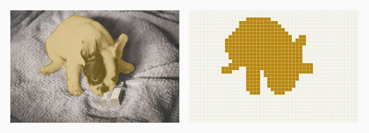
Universal architectures still trailed specialized instance systems in 2021. MaskFormer reached 40.1 instance AP with a Swin-L backbone, compared with 49.5 for Swin-HTC++ [Chen et al. 2019, Liu et al. 2021]. MaskFormer also trained for 300 epochs and its dense mask losses limited training to one image per 32 GB GPU. Mask2Former’s thesis was that the paradigm was right and the decoder and the recipe were wrong.

3. Set prediction and matching

This matching structure comes from DETR and MaskFormer. Mask2Former changes where the mask costs are evaluated, as §8 explains.

3.1 Matching as an assignment problem

The model returns a fixed set of $N$ predictions, 100 by default. Before computing the loss, it finds the lowest-cost one-to-one pairing between predictions and ground truth. The Hungarian algorithm computes this matching. The loss then scores each matched pair, while unmatched predictions are trained as no-object.

Assume an image contains at most $N$ real targets. Pad the ground truth with $\varnothing$ entries up to size $N$, so predictions and targets are both $N$-element sets. Write $\text{cost}(i, j)$ for the cost of pairing prediction $i$ with target $j$, where target $j$ carries class $c^{\text{gt}}_j$ and mask $m^{\text{gt}}_j$. The padded entries have $c^{\text{gt}}_j = \varnothing$.

$$\text{cost}(i,j) = \mathbb{1}\!\left[c^{\text{gt}}_j \ne \varnothing\right]\Big(\!-\lambda_{\text{cls}}\,\hat p_{i}(c^{\text{gt}}_j) + \lambda_{\text{ce}}\,\mathcal{L}_{\text{ce}}\big(m_{i}, m^{\text{gt}}_j\big) + \lambda_{\text{dice}}\,\mathcal{L}_{\text{dice}}\big(m_{i}, m^{\text{gt}}_j\big)\Big).$$

The minus sign favors predictions that already assign high probability to the target class. The matcher uses class probability rather than log probability. Its mask terms use the same binary cross-entropy (BCE) and Dice forms used for training. The released code solves a rectangular predictions-by-targets problem over real targets. Padding with zero-cost no-object targets gives the equivalent square matching problem used in the proof below. The classification loss later trains every unmatched prediction as no-object.

In the square view, an assignment is a permutation $\sigma \in S_N$, where $S_N$ is the set of all $N!$ reorderings. Restricted to the real targets, it pairs every target with one unique prediction. Padded targets have zero cost, so their order is irrelevant. The total cost is

$$J(\sigma) = \sum_{j=1}^{N} \text{cost}(\sigma(j),\, j),$$

and the matcher chooses $\hat\sigma = \arg\min_{\sigma} J(\sigma)$. The classic Hungarian algorithm solves this assignment problem [Kuhn 1955, Munkres 1957]. A later bookkeeping refinement brings the runtime to $O(N^3)$. The released code calls scipy.optimize.linear_sum_assignment, which uses a modified Jonker-Volgenant algorithm. The code builds the cost matrix on sampled mask points, as §8 describes.

The implementation calls scipy, but the underlying argument is useful to understand. The linear-program relaxation has an optimal permutation vertex. A companion maximization problem supplies a lower bound, and the Hungarian method reaches that bound by growing a matching on zero reduced-cost edges. The three parts are folded separately.

Why the assignment relaxation has an optimal permutation

As a linear program. Encode an assignment as $x \in \{0,1\}^{N\times N}$ with $x_{ij} = 1$ when prediction $i$ takes target $j$. Relaxing the integrality to $x \ge 0$ gives a linear program, a minimization of a linear objective over real variables subject only to linear equalities and inequalities,

$$\min_{x \ge 0}\ \sum_{i,j}\text{cost}(i,j)\,x_{ij} \quad\text{s.t.}\quad \textstyle\sum_j x_{ij} = 1\ (\forall i),\quad \sum_i x_{ij} = 1\ (\forall j).$$

The relaxation lets a prediction split fractionally across targets, which no real assignment can do. Total unimodularity guarantees that an optimal vertex is still a whole-number permutation. The next argument proves that property from the constraint matrix.

The matrix is the incidence matrix of a bipartite graph. Its rows are the $N$ prediction constraints and the $N$ target constraints, and each variable $x_{ij}$ appears in exactly two of them, prediction $i$‘s row and target $j$‘s row. So the rows carry a 2-coloring, predictions against targets, with every column showing a single 1 in each color. That structure makes the matrix totally unimodular. Every square submatrix has determinant $-1$, $0$, or $+1$.

Lemma (total unimodularity). Every square submatrix $B$ of the constraint matrix has $\det B \in \{-1, 0, +1\}$.

Proof. Induct on the order $k$ of $B$.

Base case ($k = 1$). $B$ is a single entry, $0$ or $1$, so $\det B \in \{0, 1\}$.

Inductive step ($k > 1$). Suppose the claim holds at every order below $k$. If some column of $B$ holds fewer than two 1s, take such a column. Otherwise every column holds exactly two, the most any column can carry. That gives three cases.

• Zero 1s. The column is all zeros, so $\det B = 0$.
• One 1, at row $r$, column $c$ of $B$. Laplace-expand along that column. Only the single nonzero entry contributes, so $\det B = (-1)^{r+c}\det B'$, where $B'$ deletes row $r$ and column $c$. Now $B'$ has order $k-1$, so $\det B' \in \{-1,0,1\}$ by the hypothesis, hence $\det B = \pm\det B' \in \{-1,0,1\}$.
• Two 1s in every column. Every constraint-matrix column carries its two 1s in one prediction-row and one target-row, so each column of $B$ has one 1 among the prediction-rows $P$ and one among the target-rows $T$. Summing the rows in $P$ picks up exactly one 1 per column, giving the all-ones vector $\mathbf 1$, and summing the rows in $T$ gives $\mathbf 1$ the same way. So $\sum_{r\in P} B_r - \sum_{r\in T} B_r = \mathbf 0$, a nontrivial dependence among the rows, and $B$ is singular with $\det B = 0$.

Every case lands in $\{-1,0,1\}$. $\blacksquare$

The feasible set is nonempty because it contains every permutation matrix. It is bounded because every $x_{ij}\in[0,1]$. A linear objective therefore reaches its minimum at a vertex. To see why, the Minkowski-Weyl theorem lets us write any feasible point as a convex combination $x=\sum_t\theta_t v_t$ of vertices, with $\theta_t\ge0$ and $\sum_t\theta_t=1$. Its objective value is the same weighted average of the vertex values, so it cannot beat the best vertex.

It remains to show that every vertex is integral. At a vertex, enough constraints are tight to determine the solution. The tight nonnegativity constraints hold some variables at $0$, and the surviving basic variables $x_B$ are fixed by the equality constraints. One equality is redundant because the prediction constraints and target constraints both sum to $\sum_{i,j}x_{ij}=N$. Drop it, and the remaining basis gives a square nonsingular submatrix $B$ with $Bx_B=b$, where $b$ is a vector of ones.

Cramer’s rule writes each entry of $x_B$ as a ratio of integer determinants. Total unimodularity gives $\det B=\pm1$, so every basic variable is an integer. With $x\ge0$ and every row and column summing to $1$, each row and column contains one $1$ and the rest $0$. Every vertex is therefore a permutation matrix, so the relaxation admits an optimal permutation with no rounding.

The dual certificate for optimality

The assignment minimization has a companion maximization, its dual, whose value never exceeds the original minimum. The dual attaches a potential to each constraint, $u_i$ per row and $v_j$ per column,

$$\max_{u,v\in\mathbb{R}^N}\ \sum_i u_i + \sum_j v_j \quad\text{s.t.}\quad u_i + v_j \le \text{cost}(i,j)\ (\forall i,j),$$

and dual feasibility is exactly the reduced cost $\tilde c(i,j) = \text{cost}(i,j) - u_i - v_j$ staying nonnegative everywhere.

The optimality certificate. Take any row potentials $u_1,\dots,u_N$ and column potentials $v_1,\dots,v_N$, and sum the reduced cost $\tilde c(i,j) = \text{cost}(i,j) - u_i - v_j$ along an assignment $\sigma$:

$$\begin{aligned} \sum_{j=1}^{N} \tilde c(\sigma(j),\, j) &= \sum_{j=1}^{N}\big[\text{cost}(\sigma(j),\, j) - u_{\sigma(j)} - v_j\big] && \text{definition of } \tilde c\\[2pt] &= \sum_{j=1}^{N}\text{cost}(\sigma(j),\, j) - \sum_{j=1}^{N} u_{\sigma(j)} - \sum_{j=1}^{N} v_j && \text{split the sum}\\[2pt] &= J(\sigma) - \sum_{i=1}^{N} u_i - \sum_{j=1}^{N} v_j && \text{reindex the } u \text{ sum}. \end{aligned}$$

The reindexing is legitimate because $\sigma$ is a permutation. The map $j \mapsto \sigma(j)$ hits every row index once, so $\sum_j u_{\sigma(j)} = \sum_i u_i$. The two potential sums do not depend on $\sigma$, so the potentials shift every assignment’s total by the same constant, and $\arg\min_\sigma$ is unchanged. Call the potentials feasible when $\tilde c(i,j) \ge 0$ everywhere, and an edge tight when $\tilde c(i,j) = 0$.

Lemma (a tight assignment is optimal). If feasible potentials admit an assignment $\sigma$ that uses only tight edges, then $\sigma$ minimizes $J$.

Proof. Let $\sigma'$ be any assignment. Rearranging the certificate identity,

$$\begin{aligned} J(\sigma') &= \sum_{j=1}^{N} \tilde c(\sigma'(j),\, j) + \sum_{i=1}^{N} u_i + \sum_{j=1}^{N} v_j && \text{the identity above}\\[2pt] &\ge \sum_{i=1}^{N} u_i + \sum_{j=1}^{N} v_j && \text{since every } \tilde c \ge 0. \end{aligned}$$

So $\sum_i u_i + \sum_j v_j$ lower-bounds the cost of every assignment. The tight $\sigma$ uses only edges with $\tilde c(\sigma(j),\, j) = 0$, so its first sum vanishes and $J(\sigma) = \sum_i u_i + \sum_j v_j$. That equals the lower bound, so no assignment costs less. $\blacksquare$

This equality is complementary slackness. With respect to an optimal dual solution, an optimal assignment uses only edges with $\tilde c=0$.

A worked 3×3 Hungarian run and the O(N³) bound

The primal-dual algorithm. Instead of checking all $N!$ assignments, the Hungarian method searches for feasible potentials and a complete matching on tight edges. It maintains two invariants. Reduced costs stay nonnegative, and matched edges stay tight. Consider three predictions against three targets, with prediction $i$ in row $i$, target $j$ in column $j$, and the costs collected in a matrix written $C$ for this example only.

$$C = \begin{pmatrix} 4 & 1 & 3\\ 2 & 0 & 5\\ 3 & 2 & 2 \end{pmatrix}.$$

Make zeros. Start with $u = v = 0$. Row and column reductions create enough zero reduced costs to begin matching. Subtract each row’s minimum from its row, which sets $u_i = \min_j \text{cost}(i,j)$, then subtract each remaining column minimum, $v_j = \min_i \tilde c(i,j)$. The certificate identity makes this legal because the potentials shift every assignment by the same constant. Here $u = (1, 0, 2)$ and then $v = (1, 0, 0)$.

$$\tilde c = C - u - v = \begin{pmatrix} 2 & 0 & 2\\ 1 & 0 & 5\\ 0 & 0 & 0 \end{pmatrix}.$$

A reduced cost is the pairing cost after subtracting the current row and column potentials. It measures how far an edge sits above the current dual baseline. Every row and every column now holds a zero. The column pass cannot remove a row’s zero because that zero sits in a column whose minimum is already $0$, so $v_j=0$ there and the entry stays unchanged.

Match on zeros. Pair rows to columns through tight edges only, never reusing a row or a column. Row 1 takes column 2 and row 3 takes column 1. Row 2’s only zero sits in column 2, already taken, so the matching stalls at two pairs.

The tool for getting unstuck is the augmenting path. Call a row or column free while it has no partner. An augmenting path starts at a free row, steps to a column through a zero, steps from that column to its partner row through the matched edge, steps to a new column through another zero, and keeps alternating until it lands on a free column. Flip every edge along it, matched becoming unmatched and back. Each interior row and column trades one partner for another while the two free endpoints gain one, so the matching grows by exactly one pair. Matching as far as possible means flipping augmenting paths until none exists.

None exists here. From the free row 2 the only zero leads to column 2, column 2’s partner is row 1, and row 1 owns no other zero to continue through. Dead end.

Create a new zero. The rows and columns just visited form the alternating tree, here rows $I = \{2, 1\}$ and columns $J = \{2\}$. These names are local to this example. Progress needs a zero on an edge from a row in $I$ to a column outside $J$. Take the smallest remaining reduced cost on such an edge.

$$\delta = \min_{i\in I,\ j\notin J}\tilde c(i,j) = \tilde c(2,1) = 1,$$

and pay for it with the potentials. Raise $u_i$ by $\delta$ on every tree row and lower $v_j$ by $\delta$ on every tree column. Three checks, one per kind of entry, show the move is safe.

• Tree row, outside column. The reduced cost drops by $\delta$. By the choice of $\delta$ nothing goes negative, and the minimizer lands exactly on zero. That is the purchased edge, $(2,1)$ here.
• Tree row, tree column. The raise and the drop cancel, so every edge inside the tree, the matched ones included, stays exactly as tight as it was.
• Outside row, tree column. The reduced cost rises by $\delta$, harmless for nonnegativity, and the only zeros this can erase are unmatched ones, because a tree column’s partner sits inside the tree.

So the invariants hold and the tree gains ground. The dual objective $\sum_i u_i + \sum_j v_j$ also rises by $\delta$, because the tree always holds one more row than column, every column it reaches being matched (a free column would already end an augmenting path) and each matched column bringing its partner row along, so only the root row lacks a column. The lower bound climbs toward the optimum with every lift. With $u = (2, 1, 2)$ and $v = (1, -1, 0)$,

$$\tilde c = \begin{pmatrix} 1 & 0 & 1\\ 0 & 0 & 4\\ 0 & 1 & 0 \end{pmatrix}.$$

Augment. The purchased zero at $(2,1)$ extends the search. Row 2 now reaches column 1, column 1’s partner row 3 joins, and row 3 owns a zero in column 3, which is free. That is an augmenting path, row 2 to column 1 to row 3 to column 3. Flip it. Row 2 takes column 1, row 3 moves to column 3, row 1 keeps column 2, and the matching is perfect.

Read off the certificate. In the original matrix the assignment costs $C_{12} + C_{21} + C_{33} = 1 + 2 + 2 = 5$, and the potentials sum to $(2 + 1 + 2) + (1 - 1 + 0) = 5$. Primal equals dual, so by the lemma no assignment can cost less, and enumerating all $3! = 6$ permutations confirms it. The permutation matrix of this matching is the optimal vertex of the linear program, the potentials are the optimal dual solution, and the equality that just closed is complementary slackness checked by hand. On a larger instance nothing new happens. Match through zeros until stuck, buy the cheapest escape zero, augment the moment a free column comes into reach, and stop when every row has a partner.

Each augmentation adds one edge, so at most $N$ augmentations finish the matching. One piece of bookkeeping makes each augmentation cost $O(N^2)$. For every column outside the tree, keep its current slack $\min_{i\in I}\tilde c(i,j)$ and update it in $O(N)$ when a row joins. Each $\delta$ is then read from the slacks rather than found by rescanning the matrix. Every lift either reaches a free column and enables an augmentation, or adds a matched column and its partner row to the tree. Thus at most $N$ lifts occur between augmentations, giving $O(N^3)$ work overall. The Jonker-Volgenant routine called by scipy is a faster-constant refinement of the same primal-dual idea.

The minimum assignment cost has one property the model needs.

Proposition (the matching objective ignores prediction order). Let $\mathcal{J} = \min_{\sigma\in S_N} J(\sigma)$, with the costs evaluated on the model’s current predictions. Relabeling the predictions by any permutation $\pi$ leaves $\mathcal{J}$ unchanged.

Why prediction order cannot change the matching minimum

Proof. Let $\pi \in S_N$ relabel the predictions, so that position $i$ now holds the prediction originally at position $\pi(i)$. Under the relabeling, assignment $\sigma$ pairs target $j$ with the prediction originally at position $\pi(\sigma(j))$, so its cost is

$$\sum_{j=1}^{N} \text{cost}\big(\pi(\sigma(j)),\, j\big) = J(\pi \circ \sigma) \qquad \text{(definition of } J\text{)}.$$

Minimize over $\sigma$. As $\sigma$ ranges over $S_N$, the composite $\pi \circ \sigma$ ranges over all of $S_N$ too, because left multiplication by the fixed $\pi$ is a bijection of the group, undone by composing with $\pi^{-1}$, so every $\tau \in S_N$ is hit exactly once, as $\tau = \pi \circ (\pi^{-1} \circ \tau)$. So

$$\min_{\sigma \in S_N} J(\pi \circ \sigma) = \min_{\tau \in S_N} J(\tau),$$

which is $\mathcal{J}$ before relabeling. $\blacksquare$

The minimum cost is invariant even when several assignments tie. When the optimum is unique, relabeling maps it to the corresponding relabeled assignment, so the downstream loss is unchanged. With exact cost ties, index-dependent tie-breaking can select different minimizers and therefore different gradients.

The model’s storage order carries no meaning, and the matching objective respects that. Once the assignment is fixed, it determines which target supplies each query’s training signal. §8 shows that changing only the matching cost improves AP by more than two points.

An independent nearest-target choice could assign two queries to one object and leave another unmatched. One-to-one training discourages these duplicates and enables inference without non-maximum suppression.

3.2 The training loss

Each supervised output uses classification on all $N$ queries and mask losses only on queries matched to real targets. After matching, let $y_i$ be the real class assigned to a matched query and $\varnothing$ for an unmatched query. The released criterion combines the three terms as

$$\mathcal{L} = 2\,\mathcal{L}_{\text{cls}} + 5\,\mathcal{L}_{\text{ce}} + 5\,\mathcal{L}_{\text{dice}}.$$

For one image, the classification term is weighted cross-entropy over the query slots,

$$\mathcal{L}_{\text{cls}} = \frac{\sum_{i=1}^{N} w(y_i)\big[-\log \hat p_i(y_i)\big]} {\sum_{i=1}^{N} w(y_i)}, \qquad w(y_i) = \begin{cases} 1 & y_i \ne \varnothing,\\ 0.1 & y_i = \varnothing. \end{cases}$$

The factor $2$ applies to the whole classification loss. The $0.1$ is an additional relative weight inside cross-entropy for no-object entries. In a minibatch of $B$ images, the implementation takes the same weighted mean over all $BN$ query slots. The BCE and Dice terms are averaged over the matched masks, with their point evaluations defined in §8. Their gradients explain why the two mask terms complement each other.

BCE. At a point $x$ with mask logit $z_x$, prediction $m_x = \sigma(z_x)$, and target $g_x \in \{0,1\}$, the loss is

$$\ell_{\text{ce}}(x) = -\big[g_x \log \sigma(z_x) + (1-g_x)\log\big(1-\sigma(z_x)\big)\big].$$

Its gradient through the logit collapses to one clean expression,

$$\frac{\partial \ell_{\text{ce}}}{\partial z_x} = \sigma(z_x) - g_x.$$

The BCE gradient, step by step

The two logarithms differentiate through the sigmoid, by the chain rule in the form $(\log u)' = u'/u$. With $\sigma'(z) = \sigma(z)\big(1-\sigma(z)\big)$ (differentiate $\sigma(z) = (1+e^{-z})^{-1}$ and factor the result),

$$\begin{aligned} \frac{d}{dz}\log\sigma(z) &= \frac{\sigma'(z)}{\sigma(z)} = 1 - \sigma(z) && \text{chain rule, then cancel } \sigma(z),\\[2pt] \frac{d}{dz}\log\big(1-\sigma(z)\big) &= \frac{-\sigma'(z)}{1-\sigma(z)} = -\sigma(z) && \text{chain rule, then cancel } 1-\sigma(z). \end{aligned}$$

Substitute both, then expand and cancel:

$$\begin{aligned} \frac{\partial \ell_{\text{ce}}}{\partial z_x} &= -\big[g_x\big(1 - \sigma(z_x)\big) - (1-g_x)\,\sigma(z_x)\big] && \text{substitute}\\[2pt] &= -\big[g_x - g_x\sigma(z_x) - \sigma(z_x) + g_x\sigma(z_x)\big] && \text{expand}\\[2pt] &= \sigma(z_x) - g_x && \text{cancel, then distribute the minus}. \end{aligned}$$

The gradient lies between $-1$ and $1$, and a confident error still produces a substantial update. The same expression holds for bilinearly sampled targets $g_x \in [0,1]$. The released loss averages BCE over sampled points and normalizes by the number of matched masks. BCE has no mask-level normalization for foreground area. Under dense evaluation, or uniform sampling in expectation, a large foreground contributes more positive terms for comparable pointwise errors than a small foreground. The uncertainty sampler in §8 can change those proportions by favoring logits near zero.

Dice. Mask2Former uses a soft Dice loss that normalizes overlap by predicted and target size [Milletari et al. 2016]. Write $O = \sum_x m_xg_x$ for the overlap and $S = \sum_xm_x + \sum_xg_x$ for the size sum. The released implementation is

$$\mathcal{L}_{\text{dice}}(m,g) = 1 - \frac{2O+1}{S+1}.$$

The added $1$s smooth the empty-mask case, and Milletari’s original uses sums of squares in the denominator. Dice couples all sampled points through one region-level score. Writing the smoothing constant as $\varepsilon = 1$, the gradient at a single point is

$$\frac{\partial \mathcal{L}_{\text{dice}}}{\partial m_x} = -\,\frac{2\,g_x\,(S+\varepsilon) - (2O+\varepsilon)}{(S+\varepsilon)^2}.$$

The Dice gradient, step by step

Differentiate with respect to the single probability $m_x$. Every other term of each sum is constant, so

$$\frac{\partial O}{\partial m_x} = g_x, \qquad \frac{\partial S}{\partial m_x} = 1.$$

Then, using the quotient rule in the form $(u/v)' = (u'v - uv')/v^2$,

$$\begin{aligned} \frac{\partial \mathcal{L}_{\text{dice}}}{\partial m_x} &= -\,\frac{\partial}{\partial m_x}\!\left(\frac{2O+\varepsilon}{S+\varepsilon}\right) && \text{drop the constant } 1\\[4pt] &= -\,\frac{2\,(\partial O/\partial m_x)\,(S+\varepsilon) - (2O+\varepsilon)\,(\partial S/\partial m_x)}{(S+\varepsilon)^2} && \text{quotient rule}\\[4pt] &= -\,\frac{2\,g_x\,(S+\varepsilon) - (2O+\varepsilon)}{(S+\varepsilon)^2} && \text{insert the partials}. \end{aligned}$$

When $S>0$, the unsmoothed form gives an exact view of area scaling. Tile $k$ disjoint copies of the same prediction and target pattern. Then $O$ becomes $kO$ and $S$ becomes $kS$, so the Dice value is unchanged. In the derivative above with $\varepsilon=0$, the numerator grows by $k$ while the denominator grows by $k^2$. Each copied point therefore receives $1/k$ of the original derivative. If both masks are empty, the unsmoothed ratio is undefined, which is one reason the implementation adds $1$. Dice adds a region-normalized overlap signal. It does not make the BCE component scale-invariant.

Dice pays a price one step further back, in logit space. When the prediction confidently misses the target, $m_x$ is near 0 where $g_x = 1$. The chain rule then multiplies the healthy $\partial\mathcal{L}_{\text{dice}}/\partial m_x$ by $\sigma'(z_x) \approx 0$, so the gradient dies through the saturated sigmoid. BCE cancels that factor exactly, as its logit gradient $\sigma(z_x) - g_x$ shows. BCE therefore supplies a direct logit gradient at every point, while Dice adds region-normalized overlap.

What happened to focal loss? MaskFormer used focal loss [Lin et al. 2017] with weight $20$, which down-weights already-confident predictions so easy background points contribute less. Mask2Former uses plain BCE at weight $5$. One plausible reason is that §8’s training sampler spends most of its budget on uncertain locations rather than easy background, reducing the imbalance that focal loss was designed to address. The paper does not isolate this change, so the explanation remains an inference.

The $\varnothing$ down-weighting. With $N$ queries and $T$ real segments, $N-T$ query slots are trained as no-object. Their ratio to matched slots is $(N-T)/T$. With $N=100$, this ratio is $19$ when $T=5$ and $4$ when $T=20$. Giving no-object entries a relative class weight of $0.1$ prevents the unmatched slots from overwhelming the classification term. Mask2Former inherits this weighting from DETR.

Deep supervision. The model predicts once from $\mathbf{X}_0$ and after each of nine decoder layers, giving ten supervised outputs through the same shared heads. The training objective applies the loss above to all ten. In the released criterion, Hungarian matching is recomputed for each output, so every intermediate prediction trains toward its own assignment. The thresholded intermediate masks become attention masks in §5, which makes these auxiliary losses part of the model’s feedback loop rather than an optional optimization aid.

4. The architecture

Mask2Former keeps MaskFormer’s three-part structure. A backbone produces image features. A pixel decoder turns them into a feature pyramid and a stride-4 pixel embedding map $\mathcal{E}_{\text{pixel}}$. A Transformer decoder processes $N$ queries against the image features. At any supervised output, let $q_i\in\mathbb{R}^C$ be the LayerNorm-normalized feature of query $i$. It produces a class distribution and a mask.

$$\hat p_i = \operatorname{softmax}(W_{\text{cls}}\, q_i + b_{\text{cls}}), \qquad m_i(x) = \sigma\big(\operatorname{MLP}(q_i)^\top\, \mathcal{E}_{\text{pixel}}(x)\big).$$

The class head has $W_{\text{cls}}\in\mathbb{R}^{(K+1)\times C}$ and $b_{\text{cls}}\in\mathbb{R}^{K+1}$, including one output for no-object. It predicts what the query represents. The mask MLP maps $\mathbb{R}^C$ to $\mathbb{R}^C$. Both its output and $\mathcal{E}_{\text{pixel}}(x)$ have width $C$, so their dot product produces one mask logit at pixel $x$. Masks are produced at stride 4 and then upsampled. The paper uses either a ResNet [He et al. 2016] or Swin [Liu et al. 2021] backbone. MaskFormer used a feature pyramid network (FPN) pixel decoder [Lin et al. 2017b] and six standard decoder layers over one stride-32 feature map.

5. Masked attention

Global cross-attention can learn where an object is, but the authors argue that learning this localization is slow. Masked attention starts from the region each query currently predicts and refines it layer by layer.

5.1 Why localization helps

A standard cross-attention sublayer reads the whole feature map. To keep that sublayer distinct from the complete decoder layer, write its residual state as $\widetilde{\mathbf{X}}_l$:

$$\widetilde{\mathbf{X}}_l = \operatorname{softmax}\!\big(\mathbf{Q}_l \mathbf{K}_l^{\top}\big)\,\mathbf{V}_l + \mathbf{X}_{l-1}. \tag{1}$$

Here $\mathbf{Q}_l$ comes from the previous full-layer state $\mathbf{X}_{l-1}$, while $\mathbf{K}_l$ and $\mathbf{V}_l$ come from the image features. For readability, the equation omits LayerNorm, the standard $1/\sqrt d$ scaling, the multi-head split, and the position embeddings. LayerNorm, self-attention, and the feed-forward network then turn this intermediate state into the full output $\mathbf{X}_l$. The paper writes $\mathbf{X}_l$ on the left of its simplified recurrence. The tilde here prevents that sublayer output from being confused with the complete layer output.

Nothing restricts where a query looks. Earlier DETR studies linked slow convergence to the time needed for cross-attention to become spatially focused [Gao et al. 2021, Sun et al. 2021]. Mask2Former tests the same hypothesis. In its converged cross-attention baseline, about 20 percent of the attention mass falls inside the matched ground-truth segment on COCO val. This does not show that global attention cannot localize. It shows that this baseline remains diffuse, even after training.

One toy calculation shows the effect of having many background locations. Let $n_f$ foreground locations share logit $\mu_f$, and let $n_b$ background locations share logit $\mu_b$. Their foreground attention mass is

$$\begin{aligned} \frac{n_f\, e^{\mu_f}}{n_f\, e^{\mu_f} + n_b\, e^{\mu_b}} &= \frac{1}{1 + \dfrac{n_b\, e^{\mu_b}}{n_f\, e^{\mu_f}}} && \text{divide through by } n_f\, e^{\mu_f}\\[6pt] &= \frac{1}{1 + \dfrac{n_b}{n_f}\, e^{-(\mu_f - \mu_b)}} && \text{combine the exponentials}. \end{aligned}$$

Now suppose the object covers 2 percent of the image, so $n_f = 0.02\,|\Omega|$, $n_b = 0.98\,|\Omega|$, and $n_b/n_f = 0.98/0.02 = 49$. With foreground logit margin $\mu_f - \mu_b = 2$ and $e^{-2} \approx 0.135$,

$$\frac{1}{1 + 49\,e^{-2}} \approx \frac{1}{1 + 49 \cdot 0.135} = \frac{1}{7.615} \approx 0.13.$$

In this toy model, the background wins because it has many more locations. Real attention logits are not two spikes, and sufficiently concentrated global attention can overcome the imbalance. The calculation only explains why explicit localization can make learning easier.

5.2 The masked update

Masked attention assumes that a query can update from features inside its current segment, while self-attention carries information between queries. The mask is added before the cross-attention softmax. Replacing Equation 1’s global read gives

$$\widetilde{\mathbf{X}}_l = \operatorname{softmax}\!\big(\mathcal{M}_{l-1} + \mathbf{Q}_l \mathbf{K}_l^{\top}\big)\,\mathbf{V}_l + \mathbf{X}_{l-1}, \tag{2}$$ $$\begin{aligned} B_{l-1}(i,x) &= \mathbb{1}\!\left[\sigma\!\left(\operatorname{resize}(Z_{l-1})_i(x)\right) \ge 0.5\right],\\[4pt] \mathcal{M}_{l-1}(i,x) &= \begin{cases} 0 & \text{if } B_{l-1}(i,x) = 1,\\[2pt] -\infty & \text{otherwise.} \end{cases} \end{aligned} \tag{3}$$

$Z_{l-1}$ contains the previous output’s mask logits. Each query’s logits are bilinearly resized to the current attention resolution, passed through the sigmoid, and thresholded at $0.5$ to form $B_{l-1}$. The initial logits $Z_0$ are predicted directly from the supervised learnable queries (§7).

Adding $-\infty$ before softmax gives forbidden locations zero weight and renormalizes the allowed weights to sum to 1. Zeroing weights after softmax would leave their sum below 1 unless they were normalized again. The proof is folded below.

Proposition (additive $-\infty$ masking is exact renormalization). Let $z \in \mathbb{R}^{n}$ be logits and $S \subseteq \{1,\dots,n\}$ a nonempty allowed set (an index set, not §3.2’s size sum), with $\mathcal{M}_i = 0$ for $i\in S$ and $\mathcal{M}_i = -\infty$ otherwise. Then

$$\operatorname{softmax}(z + \mathcal{M})_i = \frac{e^{z_i}\,\mathbb{1}[i\in S]}{\sum_{j\in S} e^{z_j}},$$

which is exactly the softmax of the original logits restricted to $S$.

Why masking before softmax renormalizes exactly

Proof. Fix an index $i$ and write its softmax entry from the definition:

$$\operatorname{softmax}(z + \mathcal{M})_i = \frac{e^{z_i + \mathcal{M}_i}}{\sum_{j=1}^{n} e^{z_j + \mathcal{M}_j}}.$$

Evaluate the numerator by cases, using $e^{-\infty} = 0$:

$$e^{z_i + \mathcal{M}_i} = \begin{cases} e^{z_i}\,e^{0} = e^{z_i}, & i \in S \ \ (\mathcal{M}_i = 0),\\[2pt] e^{z_i}\,e^{-\infty} = 0, & i \notin S \ \ (\mathcal{M}_i = -\infty), \end{cases}$$

so in one line the numerator is $e^{z_i}\,\mathbb{1}[i \in S]$. Split the denominator at $S$:

$$\begin{aligned} \sum_{j=1}^{n} e^{z_j + \mathcal{M}_j} &= \sum_{j\in S} e^{z_j}\,e^{0} + \sum_{j\notin S} e^{z_j}\,e^{-\infty} && \text{split over } S \text{ and its complement}\\[2pt] &= \sum_{j\in S} e^{z_j} \;>\; 0 && \text{the second sum is }0,\text{ and }S\text{ nonempty makes the first positive}. \end{aligned}$$

Divide numerator by denominator:

$$\operatorname{softmax}(z + \mathcal{M})_i = \frac{e^{z_i}\,\mathbb{1}[i \in S]}{\sum_{j\in S} e^{z_j}},$$

the softmax of the original logits restricted to $S$. $\blacksquare$

The paper’s R50 ablation on COCO compares four updates. Plain cross-attention reaches 37.8 AP, spatially modulated co-attention (SMCA) [Gao et al. 2021] reaches 37.9, mask pooling reaches 43.1, and masked attention reaches 43.7. Mask pooling averages the features inside a mask. Masked attention still learns a distribution within the allowed region.

Additive attention masking already existed in Transformer decoders [Vaswani et al. 2017]. Mask2Former makes the mask spatial, query-specific, and dependent on the previous mask prediction. The prediction restricts the next read, and the next query state produces a new prediction.

5.3 Gradients and empty masks

The attention gate is Boolean, so gradients do not pass through the threshold. Intermediate masks instead learn from the per-layer auxiliary losses in §3.2. Those losses compare each intermediate prediction directly with the target mask. On a binary target grid, the gate becomes correct as soon as every prediction falls on the right side of $0.5$. The exact statement and the boundary caveat are folded below.

When mask supervision gives the correct binary gate

First assume the evaluated targets are binary. As a function of probability on the closed interval $[0,1]$, BCE is minimized pointwise at $m_x=g_x$. A finite sigmoid output lies in $(0,1)$, so the logit-parameterized loss approaches this endpoint infimum as $z_x\to+\infty$ for $g_x=1$ or $z_x\to-\infty$ for $g_x=0$. For soft Dice,

$$2\sum_x m_x g_x \le \sum_x m_x + \sum_x g_x,$$

because for $m_x\in[0,1]$ and binary $g_x$,

$$m_x + g_x - 2m_xg_x = m_x(1-g_x) + g_x(1-m_x) \ge 0.$$

Equality holds only when $m_x=g_x$ at every evaluated binary point, so soft Dice also has its closed-domain minimum of zero only at the target mask. Finite sigmoid logits approach that endpoint solution rather than attaining it exactly.

The released sampler reads the ground-truth mask with bilinear interpolation. Points near a boundary can therefore have fractional targets $g_x\in(0,1)$. BCE is still minimized at that fractional value, but the Dice equality argument above no longer applies pointwise. The proof is exact on the binary grid and explains why direct mask supervision is aligned with the gate. It is not a proof that the sampled BCE-plus-Dice objective has its minimum at every fractional boundary value.

The thresholded gate needs less than exact probability convergence. If $g_x=1$ and $|m_x-g_x|<0.5$, then $m_x>0.5$. If $g_x=0$ under the same condition, then $m_x<0.5$. Every gate decision is therefore correct once the pointwise errors are below $0.5$.

The implementation also guards against an empty predicted region. If a query’s thresholded mask is empty at some scale, every attention logit would be $-\infty$ and softmax would be undefined. The code makes each affected row fully unmasked for one layer. The exact guard and its reason are folded below.

How the implementation handles an empty attention mask

attn_mask = (mask_logits.sigmoid() < 0.5).flatten(2)   # True = forbidden
attn_mask[attn_mask.all(dim=-1)] = False               # Fall back to global attention.

Without the guard, the row’s softmax denominator is zero, which can introduce a NaN. The following self-attention mixes information across queries, so that invalid value can contaminate other query states, the loss, and the gradients. Flipping the row to fully unmasked also keeps the §5.2 proposition’s hypothesis true. Its allowed set $S$ becomes the whole grid rather than the empty set.

5.4 Did it work?

In the supplementary analysis, average attention mass inside the matched foreground rises from about 0.20 to 0.59. One masked-attention layer also outperforms nine standard cross-attention layers on PQ in the reported layer-wise comparison. Removing masked attention costs 5.9 AP, 4.8 PQ, and 1.7 mIoU. This is the largest drop in the paper’s ablations.

6. Feeding the decoder

6.1 The cost structure

Cross-attention cost grows with the number of image tokens. Its main attention operations cost $O(NH_lW_lC)$ for $N$ queries, an $H_l$ by $W_l$ feature map, and channel width $C$. For a 1024 by 1024 input, strides 32, 16, and 8 contain 1,024, 4,096, and 16,384 tokens. The finest map therefore costs about sixteen times more to attend over than the coarsest.

6.2 The schedule

Mask2Former reads one scale per decoder layer. Layers 1, 2, and 3 use strides 32, 16, and 8, and the cycle repeats twice more. Feeding all three scales to every layer reaches 44.0 AP at 247 GFLOPs. Using only stride 8 reaches the same AP at 239 GFLOPs. The round-robin schedule reaches 43.7 AP at 226 GFLOPs, trading 0.3 AP for lower cost. Removing high-resolution features lowers AP by 2.2.

Each feature also receives DETR’s two-dimensional sinusoidal position encoding and a learned embedding that identifies its scale. The position coordinates are normalized per axis before the sine and cosine features are formed. The scale embedding follows Deformable DETR [Zhu et al. 2021].

6.3 The pixel decoder

The default pixel decoder has six multi-scale deformable-attention (MSDeformAttn) layers over strides 8, 16, and 32. It then fuses the result with stride-4 backbone features to produce pixel embeddings. Each location samples a small learned set of points from every feature level instead of attending densely to all locations [Zhu et al. 2021]. The exact operator and cost are folded below.

The MSDeformAttn operator and its cost

For feature $z_q$ at normalized reference point $\hat p_q$,

$$\text{MSDeformAttn}\big(z_q, \hat p_q, \{x^l\}\big) = \sum_{m=1}^{M} W_m \Big[ \sum_{l=1}^{L}\sum_{k=1}^{P} A_{mlqk}\; W'_m\, x^l\big(\psi_l(\hat p_q) + \Delta p_{mlqk}\big) \Big].$$

Here $m$, $l$, and $k$ index the $M$ heads, $L$ levels, and $P$ sample points per level, and $x^l$ is the feature map at level $l$. This $M$ counts heads, not masks. $W'_m$ projects values into head $m$, $W_m$ projects that head back to width $C$, and $\psi_l$ maps the normalized reference point into level $l$. The two-dimensional offsets $\Delta p_{mlqk}\in\mathbb{R}^2$ and nonnegative weights $A_{mlqk}$ are predicted from $z_q$, with $\sum_{l,k}A_{mlqk}=1$ for each head $m$ and query $q$. Bilinear interpolation reads fractional locations, and samples outside a feature map contribute zero. The aggregation processes $M\!\times\!L\!\times\!P$ entries of width $C/M$, so it costs $O(LPC)$ per query apart from the learned projections. Dense attention would read every location at every level.

Among conventional pyramid decoders, BiFPN has the highest AP at 43.5 and ties FaPN at 51.8 PQ. FaPN has the highest mIoU at 46.8 [Tan et al. 2020, Huang et al. 2021]. MSDeformAttn is higher on all three at 43.7 AP, 51.9 PQ, and 47.2 mIoU.

7. Rewiring the decoder layer

Mask2Former changes the decoder layer in three ways without adding FLOPs. Together they improve AP by about 1.4, PQ by 1.1, and mIoU by 0.9. Their effects overlap, so the one-at-a-time ablations in §11 do not add to those totals.

Masked attention comes first. The standard order is self-attention, then cross-attention, then the feed-forward network. Mask2Former uses masked attention, then self-attention, then the feed-forward network. Running cross-attention first gives each query image context before the queries interact. Restoring the original order costs 0.5 AP.

Query features are learnable and directly supervised. DETR zero-initializes query features and learns only positional embeddings. Mask2Former makes $\mathbf{X}_0$ learnable and supervises its masks before the decoder runs. The query positional embeddings stay learnable, as in DETR. Every decoder layer adds them to the query features when computing attention, and they appear as query_pos in the appendix. Direct supervision also gives the first layer a useful gate.

Without direct supervision, learnable queries match zero initialization on AP and PQ but improve mIoU from 45.5 to 47.0. Adding supervision reaches 43.7 AP, 51.9 PQ, and 47.2 mIoU. The paper compares the supervised initial predictions to region proposals [Ren et al. 2015] that the decoder refines.

Dropout is removed. Restoring dropout lowers AP by 0.7 and PQ by 0.6 in the ablation.

8. Matching and training on points

8.1 The memory problem and the estimator

Dense mask losses are expensive. Mask2Former evaluates them at sampled coordinates instead. Uniform points build matching costs, while prediction-dependent uncertain points train matched masks.

MaskFormer computed dense mask costs for every prediction-target pair and dense losses again for matched pairs at every supervised head. This limited training to one image per 32 GB GPU. Following PointRend [Kirillov et al. 2020], Mask2Former evaluates these terms at $K_{\text{pt}} = 12{,}544 = 112^2$ sampled points.

The implementation samples normalized continuous coordinates. At coordinate $u$, it bilinearly interpolates the prediction logit map $Z$ and target mask $G$:

$$z(u)=\operatorname{bilinear}(Z,u), \qquad g(u)=\operatorname{bilinear}(G,u).$$

BCE is applied directly to $z(u)$ with target $g(u)$. Dice first applies $\sigma$ to $z(u)$. This order matters because $\sigma(\operatorname{bilinear}(Z,u))$ is not generally equal to bilinear interpolation of $\sigma(Z)$. For an additive point loss such as BCE, the mean over uniform samples is an unbiased estimate of the spatial average, and its variance falls as $1/K_{\text{pt}}$. The derivation is folded below.

Why uniform points are unbiased for additive losses

Condition on the current prediction logits and target mask. Let $u_1,\dots,u_{K_{\text{pt}}}$ be independent uniform points in the unit square, and let $\ell(u)$ be any additive loss evaluated from $z(u)$ and $g(u)$, with finite variance. For BCE, $\ell(u)$ is the numerically stable BCE-with-logits loss. The Monte Carlo average is

$$\hat{\mathcal{L}} = \frac{1}{K_{\text{pt}}}\sum_{k=1}^{K_{\text{pt}}}\ell(u_k)$$

The expectation $\mathbb{E}$ is the average over repeated point draws, and the variance $\operatorname{Var}$ measures how much the estimate changes between draws. Linearity of expectation gives the spatial mean. Independence removes the covariance terms in the variance.

$$\mathbb{E}[\hat{\mathcal{L}}] = \frac{1}{K_{\text{pt}}}\sum_k \mathbb{E}[\ell(u_k)] = \int_{[0,1]^2}\ell(u)\,du, \qquad \operatorname{Var}[\hat{\mathcal{L}}] = \frac{1}{K_{\text{pt}}}\operatorname{Var}[\ell(u_1)].$$

This is unbiased for the continuous bilinear-sampling objective $\int_{[0,1]^2}\ell(u)\,du$, which need not equal the arithmetic mean over raster pixels. In the released criterion, target masks are padded to the batch shape and the returned validity mask is not applied, so sampled padded areas remain part of that implementation objective. The unbiased statement applies to additive point losses. Dice is a ratio of sampled sums, so its sampled value is not unbiased in general. The code and the paper rely on the empirical result in the §8.3 ablation rather than an exact equivalence proof.

8.2 Two sampling rules for two jobs

The two sampling rules serve different parts of training.

Matching uses shared uniform points. One set of normalized coordinates is sampled uniformly and reused for every prediction and target mask in the image. Reuse makes the cost matrix cheaper to build. A conditional variance argument for shared samples is folded below. It is not a claim made by the paper.

When shared points reduce comparison variance

Let $A$ and $B$ be two additive cost estimates evaluated on the same $K_{\text{pt}}$ uniform points. Covariance measures whether the two estimates move together across repeated draws. Then

$$\operatorname{Var}[A-B] = \operatorname{Var}[A]+\operatorname{Var}[B]-2\operatorname{Cov}(A,B).$$

Independent point sets make the covariance term zero. Shared points can make it positive because both estimates respond to the same sampled locations. When it is positive, the variance of the difference falls. When it is negative, the variance rises. The equation gives a condition under which sharing stabilizes a comparison. It does not prove that every matching comparison becomes more stable.

Training uses uncertain points. For each matched mask, the PointRend sampler draws $3K_{\text{pt}}$ uniform candidates [Kirillov et al. 2020]. It keeps the $0.75K_{\text{pt}}$ candidates whose prediction logits are closest to zero, then adds $0.25K_{\text{pt}}$ fresh uniform points. The uncertainty score depends on the prediction, not the ground truth. These points often lie near a predicted boundary, but uncertain interiors can also be selected.

This training sampler is intentionally nonuniform and applies no importance correction. Its selected coordinates are treated as fixed when gradients are computed, so it does not provide an unbiased estimate of the dense loss. Instead, it concentrates the stochastic training signal on uncertain regions. The §8.3 ablation shows that this signal preserves performance while reducing memory.

8.3 Point-sampling ablation

matching on	training loss on	AP (COCO)	PQ (COCO)	mIoU (ADE20K)	memory
masks	masks	41.0	50.3	45.9	18 GB
masks	points	41.0	50.8	45.9	6 GB
points	masks	43.1	51.4	47.3	18 GB
points	points	43.7	51.9	47.2	6 GB

Using points for the training loss reduces reported training memory from 18 GB to 6 GB in the paper’s R50 COCO ablation. AP and mIoU stay the same in the dense-matching rows, while PQ rises from 50.3 to 50.8. Using points for matching raises AP from 41.0 to 43.1 with dense training, then to 43.7 with point training. The table measures the effect. Why point-based matching improves the assignment is left open.

9. Training recipe

The table compares Mask2Former’s training recipe with MaskFormer’s. In the decoder row, SA, CA, and MA abbreviate self-attention, cross-attention, and masked attention.

	MaskFormer	Mask2Former
optimizer	AdamW [Loshchilov & Hutter 2019], lr $10^{-4}$	AdamW, lr $10^{-4}$
weight decay	$10^{-4}$	0.05
backbone lr multiplier	0.1 (CNN backbones)	0.1 (CNN and Transformer backbones)
schedule (COCO)	300 epochs at batch 64	50 epochs at batch 16, lr ×0.1 at 90% and 95% of steps
augmentation	standard scale and crop	LSJ (large-scale jittering) [Ghiasi et al. 2021], scale 0.1 to 2.0 with a fixed $1024^2$ crop
mask loss	focal ($\lambda{=}20$) + dice ($\lambda{=}1$), dense	BCE ($\lambda{=}5$) + dice ($\lambda{=}5$) on 12,544 points
$\lambda_{\text{cls}}$	1.0	2.0, with a 0.1 no-object multiplier
decoder	6 layers, SA→CA→FFN, dropout 0.1, stride 32 only, zero-init queries	9 layers, MA→SA→FFN, no dropout, strides {32,16,8}×3, learnable supervised queries

COCO inference resizes the shorter image side to 800 pixels and caps the longer side at 1333. Most models use 100 queries. The largest panoptic and instance models use 200. In the R50 ablation, 100 queries gives the best AP and mIoU, while 200 raises PQ from 51.9 to 52.2. The best setting depends on how many segments an image contains.

Training settings beyond COCO

Cityscapes [Cordts et al. 2016] uses 90,000 iterations with 512 by 1024 crops. ADE20K [Zhou et al. 2017] uses 640 by 640 crops for panoptic and instance training. Semantic crop size varies by backbone. Mapillary Vistas [Neuhold et al. 2017] uses 300,000 iterations with 1024 by 1024 crops.

Post-processing follows MaskFormer. Semantic output sums the masks weighted by each class probability, then selects the highest-scoring class at every pixel.

Panoptic output first keeps queries whose best class is not no-object and whose class probability exceeds $0.8$. Each pixel chooses the kept query with the largest class-probability times mask-probability score. The pixel is written only if the winning query’s mask probability is at least $0.5$. For each query, the code divides the number of pixels it wins by the number of pixels in its own thresholded mask and discards the segment when this ratio is below $0.8$. The final segment is the intersection of the winning pixels and that thresholded mask. Stuff segments with the same class are merged. Rejected pixels remain void.

Instance output flattens the $N\times K$ query-class probabilities and selects the highest-scoring pairs. The released code keeps the top 100 pairs per image. The same query mask can therefore appear with more than one class before the top-pair cutoff. For a selected pair $(i,c)$, the final score multiplies its class probability by the average mask probability over the predicted foreground.

$$s_{i,c} = \hat p_i(c)\, \frac{\sum_x m_i(x)\,\mathbb{1}[m_i(x)>0.5]} {\sum_x \mathbb{1}[m_i(x)>0.5] + \varepsilon}.$$

The implementation uses $\varepsilon = 10^{-6}$, so an empty foreground scores zero.

10. Results

The largest models reported in the paper achieve the following results.

task / dataset	Mask2Former (Swin-L)	previous best	margin
Panoptic, COCO val	57.8 PQ	MaskFormer 52.7, K-Net 54.6	+5.1 / +3.2
Instance, COCO val	50.1 AP (36.2 boundary AP)	Swin-HTC++ 49.5 (34.1)	+0.6 (+2.1)
Semantic, ADE20K val	57.7 mIoU (Swin-L, FaPN, multi-scale inference)	BEiT 57.0	+0.7 at less than half the parameters

Boundary AP uses the minimum of mask IoU and Boundary IoU [Cheng et al. 2021c]. Multi-scale in the semantic row means test-time inference over several input sizes. It is unrelated to the decoder schedule. The 57.7 mIoU model also uses FaPN instead of the default MSDeformAttn pixel decoder.

With ResNet-50, Mask2Former reaches 51.9 PQ after 50 epochs. MaskFormer reports 46.5 after 300 epochs. The comparison includes architecture, loss, augmentation, batch size, and optimizer-setting changes, so it should not be read as a controlled convergence experiment. The paper’s appendix isolates one of these variables. Trained with standard augmentation instead of LSJ, R50 Mask2Former converges in 25 epochs, so the short schedule is not an artifact of the augmentation.

The detailed results show three contrasts. Large-object AP reaches 71.2 on COCO test-dev, while small-object AP reaches 29.1. COCO assigns size buckets by mask area. Small means below $32^2$ pixels and large means above $96^2$ pixels.

Boundary AP improves by 2.1 over HTC++, compared with 0.6 overall. The larger Boundary AP gain shows better boundary accuracy, but the comparison does not isolate its cause.

Swin-T Mask2Former reaches 53.2 PQ at 232 GFLOPs, while Swin-L MaskFormer reaches 52.7 at 792 GFLOPs. Throughput moves the other way. The R50 panoptic model runs at 8.6 frames per second, compared with MaskFormer’s 17.6.

The architecture is also evaluated on Cityscapes, ADE20K, and Mapillary Vistas. A Swin-L panoptic checkpoint reaches 66.6 PQ and 43.6 $\text{AP}^{\mathrm{Th}}_{\mathrm{pan}}$ on Cityscapes, the instance AP on thing classes computed from the panoptic checkpoint. The separate Cityscapes instance checkpoint reaches 43.7 AP. Swin-L panoptic checkpoints reach 48.1 PQ on ADE20K and 45.5 PQ on Mapillary Vistas. Each checkpoint is trained for its dataset and task.

11. Ablations and interactions

The table reports controlled R50 ablations across all three tasks.

change (removed or varied)	ΔAP	ΔPQ	ΔmIoU	takeaway
remove masked attention	−5.9	−4.8	−1.7	largest measured drop
remove multi-scale high-res features	−2.2	−1.7	−1.1	finer features matter
replace point matching with dense masks	−2.7	−1.1	−1.3*	point matching improves all three tasks
replace supervised learnable features with zero-init	−0.8	−0.7	−1.8	direct supervision of initial queries matters
restore dropout	−0.7	−0.6	0.0	dropout hurts AP and PQ in this setup
vanilla layer order	−0.5	−0.3	−0.9	masked attention first performs better

*Measured with point-sampled training loss fixed. The full two-by-two comparison appears in §8.3.

The sequential substitutions show how the complete system was assembled. Retraining MaskFormer with Mask2Former’s recipe raises AP from 34.0 to 37.8. Replacing the decoder raises it to 41.5. Replacing the FPN pixel decoder with MSDeformAttn reaches 43.7. These increments are not independent causal shares. The components interact, and a different substitution order could produce different gains.

12. Limitations

Universal means one architecture, not one checkpoint. The paper trains separate models for each dataset and task. A panoptic COCO checkpoint reaches 41.7 instance AP, compared with 43.7 for instance-specific training. Its semantic score is 61.7 mIoU, compared with 61.5 for semantic-specific training. Results differ across ADE20K and Cityscapes, so panoptic training does not consistently replace task-specific training.

Small objects remain weaker. Small-object AP is 29.1, compared with 71.2 for large objects. The paper lists fuller use of the feature pyramid as future work. Mask2Former is also slower than MaskFormer, and its query count must be chosen for the expected number of segments.

13. Later work

The same group extended Mask2Former to video instance segmentation [Cheng et al. 2021b]. OneFormer [Jain et al. 2023] trains one task-conditioned model for all three image segmentation tasks. Mask DINO [Li et al. 2023] combines mask prediction with DETR-style detection. These models keep the query-based mask-classification structure while changing the training objective or supported outputs.

14. Conclusion

Mask2Former works because its changes form a feedback loop. Matching assigns one target to each query. Deep supervision trains every intermediate mask. Each mask restricts the next cross-attention step, and point sampling makes this repeated supervision affordable. The ablation gains in §11 overlap because these parts depend on one another.

Later systems changed the objectives and supported outputs but kept this query-to-mask refinement loop. That loop, rather than any one benchmark result, is Mask2Former’s lasting contribution.

Appendix A. Implementation notes

The reference implementation is facebookresearch/Mask2Former, built on Detectron2 [Wu et al. 2019]. It was archived on January 1, 2025. Hugging Face provides Mask2FormerForUniversalSegmentation with Mask2FormerImageProcessor or AutoImageProcessor. The image processor exposes semantic, instance, and panoptic post-processing methods. The decoder core is shown below in simplified PyTorch-style pseudocode.

def decoder_layer(
    x, feats_l, size_l, pos_l, lvl_emb, query_pos,
    prev_mask_logits, pixel_embeddings, num_heads,
):
    # x: (N,B,C) · feats_l: (H_l*W_l,B,C) · size_l: (H_l,W_l)
    m = F.interpolate(
        prev_mask_logits,
        size=size_l,
        mode="bilinear",
        align_corners=False,
    )
    attn_mask = (m.sigmoid() < 0.5).flatten(2)  # (B,N,H_l*W_l)
    attn_mask = attn_mask[:, None].repeat(
        1, num_heads, 1, 1
    ).flatten(0, 1).detach()                     # (B*num_heads,N,H_l*W_l)
    attn_mask[attn_mask.all(dim=-1)] = False    # Prevent all-masked softmax.

    # The scale embedding is part of both the key and value memory.
    feats_l = feats_l + lvl_emb
    x = norm1(x + cross_attn(
        q=with_pos(x, query_pos),
        k=with_pos(feats_l, pos_l),
        v=feats_l,
        attn_mask=attn_mask,
    ))
    x = norm2(x + self_attn(
        q=with_pos(x, query_pos),
        k=with_pos(x, query_pos),
        v=x,
    ))
    x = norm3(x + ffn(x))

    h = decoder_norm(x).transpose(0, 1)
    cls_logits = class_head(h)
    mask_logits = einsum(
        "bnc,bchw->bnhw", mask_head(h), pixel_embeddings
    )
    return x, cls_logits, mask_logits

The heads run once on $\mathbf{X}_0$ before the loop and after each of nine decoder layers. The initial prediction supplies $Z_0$. The final output receives the main loss, and the preceding nine outputs receive auxiliary losses.

Appendix B. Questions and answers

These questions revisit the main arguments. Each answer is folded so the prompt can be used as a check before opening it.

Why must masking happen before softmax?

Adding $-\infty$ before softmax makes $e^{z+\mathcal{M}}$ vanish outside the allowed set $S$. The remaining weights form a restricted softmax and still sum to 1. Zeroing entries after softmax leaves coefficients whose sum is below 1 unless they are normalized again. This does not imply that the resulting vector norm always shrinks.

What is the toy foreground share at 2 percent coverage and margin 2?

For foreground fraction $\rho$ and logit margin $\Delta$, the two-logit model gives

$$\text{share} = \frac{1}{1 + \dfrac{1-\rho}{\rho}e^{-\Delta}}.$$

At $\rho=0.02$ and $\Delta=2$, this is $1/(1+49e^{-2})\approx0.13$. It is a toy-model result, not a prediction for real attention distributions.

Why can prediction order not change the matching minimum?

Relabeling by $\pi$ turns the cost of assignment $\sigma$ into the cost of $\pi\circ\sigma$. Composition with a fixed permutation is a bijection of $S_N$, so the minimum is unchanged. When the optimum is unique, relabeling maps it to the corresponding relabeled assignment and the downstream loss is unchanged. With exact ties, index-dependent tie-breaking can select different minimizers and therefore different gradients.

How do thresholded gates learn without gate gradients?

They do not learn through the Boolean gate. Per-layer deep supervision trains every intermediate mask directly. Section 5.3 states precisely when this supervision gives the correct binary gate and explains the caveat introduced by fractional boundary samples.

Why do matching and training use different point samplers?

Sharing one uniform coordinate set makes the matching cost matrix efficient to build. For additive losses, each entry estimates the continuous bilinear-sampling objective. Training instead favors prediction logits near zero and keeps a random fraction for spatial coverage. The uncertain sampler does not use the target mask.

What do the larger AP and PQ gains show?

The ablation shows a larger gain for instance and panoptic segmentation than for semantic segmentation. Identity separation is a plausible explanation, but the experiment cannot isolate it as the cause.

How do overlapping masks become a panoptic partition?

Post-processing in §9 imposes exclusivity. Panoptic inference keeps confident non-no-object queries and finds each pixel’s strongest query. It writes the pixel only when the winning mask probability is at least $0.5$, applies the $0.8$ overlap filter, and merges same-class stuff. Rejected pixels remain void. The surviving segments do not overlap.

Why does greedy matching work for PQ but not for training?

The §1 lemma proves uniqueness for non-overlapping segments above $0.5$ IoU. Training predictions can overlap and use soft costs, so they still require an assignment algorithm.

References

1. Cheng, Misra, Schwing, Kirillov, Girdhar. “Masked-attention Mask Transformer for Universal Image Segmentation.” CVPR 2022. Paper · Supplement · Code
2. Cheng, Schwing, Kirillov. “Per-Pixel Classification is Not All You Need for Semantic Segmentation.” NeurIPS 2021. arXiv:2107.06278
3. Carion, Massa, Synnaeve, Usunier, Kirillov, Zagoruyko. “End-to-End Object Detection with Transformers.” ECCV 2020. arXiv:2005.12872
4. Kirillov, He, Girshick, Rother, Dollár. “Panoptic Segmentation.” CVPR 2019. arXiv:1801.00868
5. Kirillov, Wu, He, Girshick. “PointRend: Image Segmentation as Rendering.” CVPR 2020. arXiv:1912.08193
6. Zhu, Su, Lu, Li, Wang, Dai. “Deformable DETR.” ICLR 2021. arXiv:2010.04159
7. Zhang, Pang, Chen, Loy. “K-Net: Towards Unified Image Segmentation.” NeurIPS 2021. arXiv:2106.14855
8. Wang, Zhu, Adam, Yuille, Chen. “MaX-DeepLab: End-to-End Panoptic Segmentation with Mask Transformers.” CVPR 2021. arXiv:2012.00759
9. He, Gkioxari, Dollár, Girshick. “Mask R-CNN.” ICCV 2017. arXiv:1703.06870
10. Long, Shelhamer, Darrell. “Fully Convolutional Networks for Semantic Segmentation.” CVPR 2015. arXiv:1411.4038
11. Vaswani et al. “Attention Is All You Need.” NeurIPS 2017. arXiv:1706.03762
12. Kuhn. “The Hungarian Method for the Assignment Problem.” Naval Research Logistics Quarterly, 1955.
13. Munkres. “Algorithms for the Assignment and Transportation Problems.” Journal of the SIAM, 1957.
14. Milletari, Navab, Ahmadi. “V-Net: Fully Convolutional Neural Networks for Volumetric Medical Image Segmentation.” 3DV 2016. arXiv:1606.04797
15. Lin, Goyal, Girshick, He, Dollár. “Focal Loss for Dense Object Detection.” ICCV 2017. arXiv:1708.02002
16. Lin, Dollár, Girshick, He, Hariharan, Belongie. “Feature Pyramid Networks for Object Detection.” CVPR 2017. arXiv:1612.03144
17. Gao, Zheng, Wang, Dai, Li. “Fast Convergence of DETR with Spatially Modulated Co-Attention.” ICCV 2021. arXiv:2101.07448
18. Sun, Cao, Yang, Kitani. “Rethinking Transformer-based Set Prediction for Object Detection.” ICCV 2021. arXiv:2011.10881
19. Liu et al. “Swin Transformer: Hierarchical Vision Transformer using Shifted Windows.” ICCV 2021. arXiv:2103.14030
20. He, Zhang, Ren, Sun. “Deep Residual Learning for Image Recognition.” CVPR 2016. arXiv:1512.03385
21. Chen et al. “Hybrid Task Cascade for Instance Segmentation.” CVPR 2019. arXiv:1901.07518
22. Ren, He, Girshick, Sun. “Faster R-CNN.” NeurIPS 2015. arXiv:1506.01497
23. Tan, Pang, Le. “EfficientDet: Scalable and Efficient Object Detection.” CVPR 2020. arXiv:1911.09070
24. Huang, Lu, Cheng, He. “FaPN: Feature-Aligned Pyramid Network for Dense Image Prediction.” ICCV 2021. arXiv:2108.07058
25. Loshchilov, Hutter. “Decoupled Weight Decay Regularization.” ICLR 2019. arXiv:1711.05101
26. Ghiasi et al. “Simple Copy-Paste is a Strong Data Augmentation Method for Instance Segmentation.” CVPR 2021. arXiv:2012.07177
27. Chen, Papandreou, Kokkinos, Murphy, Yuille. “DeepLab: Semantic Image Segmentation with Deep Convolutional Nets, Atrous Convolution, and Fully Connected CRFs.” TPAMI 2018. arXiv:1606.00915
28. Zhao, Shi, Qi, Wang, Jia. “Pyramid Scene Parsing Network.” CVPR 2017. arXiv:1612.01105
29. Wang, Girshick, Gupta, He. “Non-local Neural Networks.” CVPR 2018. arXiv:1711.07971
30. Fu et al. “Dual Attention Network for Scene Segmentation.” CVPR 2019. arXiv:1809.02983
31. Strudel, Garcia, Laptev, Schmid. “Segmenter: Transformer for Semantic Segmentation.” ICCV 2021. arXiv:2105.05633
32. Xie et al. “SegFormer: Simple and Efficient Design for Semantic Segmentation with Transformers.” NeurIPS 2021. arXiv:2105.15203
33. Bao, Dong, Wei. “BEiT: BERT Pre-Training of Image Transformers.” ICLR 2022. arXiv:2106.08254
34. Everingham et al. “The PASCAL Visual Object Classes Challenge: A Retrospective.” IJCV 2015.
35. Lin et al. “Microsoft COCO: Common Objects in Context.” ECCV 2014. arXiv:1405.0312
36. Cordts et al. “The Cityscapes Dataset for Semantic Urban Scene Understanding.” CVPR 2016.
37. Zhou et al. “Scene Parsing through ADE20K.” CVPR 2017.
38. Neuhold, Ollmann, Rota Bulò, Kontschieder. “The Mapillary Vistas Dataset for Semantic Understanding of Street Scenes.” ICCV 2017.
39. Cheng et al. “Mask2Former for Video Instance Segmentation.” 2021. arXiv:2112.10764
40. Jain et al. “OneFormer: One Transformer to Rule Universal Image Segmentation.” CVPR 2023. arXiv:2211.06220
41. Li et al. “Mask DINO: Towards a Unified Transformer-based Framework for Object Detection and Segmentation.” CVPR 2023. arXiv:2206.02777
42. Wu, Kirillov, Massa, Lo, Girshick. “Detectron2.” 2019. github.com/facebookresearch/detectron2
43. Cheng, Girshick, Dollár, Berg, Kirillov. “Boundary IoU: Improving Object-Centric Image Segmentation Evaluation.” CVPR 2021. arXiv:2103.16562

Citation

Suggested citation

Massih, Peter. “Mask2Former, Dissected.” Peter’s Patches, no. 1, Jul 2026. https://peteramassih.com/writing/mask2former.

BibTeX

@article{massih2026mask2former,
  title   = {Mask2Former, Dissected},
  author  = {Massih, Peter},
  journal = {peteramassih.com},
  series  = {Peter's Patches},
  number  = {1},
  year    = {2026},
  month   = {July},
  url     = {https://peteramassih.com/writing/mask2former}
}